Everything You Need to Know About Linear Functions and Modeling Linear Functions
4.iii: Modeling with Linear Functions
- Folio ID
- 15063

Learning Objectives
- Build linear models from exact descriptions.
- Model a set of data with a linear function.
Emily is a higher pupil who plans to spend a summer in Seattle. She has saved $3,500 for her trip and anticipates spending $400 each week on hire, nutrient, and activities. How can we write a linear model to stand for her situation? What would be the 10-intercept, and what tin she learn from it? To answer these and related questions, we can create a model using a linear function. Models such equally this one can be extremely useful for analyzing relationships and making predictions based on those relationships. In this section, we will explore examples of linear function models.

Identifying Steps to Model and Solve Bug
When modeling scenarios with linear functions and solving problems involving quantities with a abiding rate of change, we typically follow the aforementioned problem strategies that we would use for any blazon of function. Let's briefly review them:
Identify irresolute quantities, and and then ascertain descriptive variables to correspond those quantities. When appropriate, sketch a picture or define a coordinate organisation.
Advisedly read the problem to identify important data. Look for information that provides values for the variables or values for parts of the functional model, such as slope and initial value.
Carefully read the trouble to decide what we are trying to find, identify, solve, or interpret.
Identify a solution pathway from the provided information to what we are trying to detect. Oft this volition involve checking and tracking units, building a tabular array, or fifty-fifty finding a formula for the function being used to model the trouble.
When needed, write a formula for the function.
Solve or evaluate the function using the formula.
Reverberate on whether your answer is reasonable for the given situation and whether information technology makes sense mathematically.
Conspicuously convey your result using appropriate units, and reply in total sentences when necessary.
Edifice Linear Models
Now allow's take a look at the student in Seattle. In her situation, at that place are two changing quantities: time and money. The corporeality of money she has remaining while on vacation depends on how long she stays. Nosotros can use this data to define our variables, including units.
- Output: \(Thou\), money remaining, in dollars
- Input: \(t\), fourth dimension, in weeks
Then, the amount of money remaining depends on the number of weeks: \(Yard(t)\)
We can also identify the initial value and the rate of change.
- Initial Value: She saved $three,500, so $3,500 is the initial value for M.
- Rate of Change: She anticipates spending $400 each calendar week, then –$400 per week is the rate of modify, or slope.
Notice that the unit of dollars per calendar week matches the unit of measurement of our output variable divided by our input variable. Also, because the slope is negative, the linear role is decreasing. This should make sense because she is spending money each week.
The charge per unit of modify is abiding, then we tin can start with the linear model \(Thousand(t)=mt+b\). Then we can substitute the intercept and gradient provided.

To find the ten-intercept, we set the output to zero, and solve for the input.
\[\begin{align*} 0&=−400t+3500 \\ t&=\dfrac{3500}{400} \\ &=8.75 \end{align*}\]
The x-intercept is 8.75 weeks. Because this represents the input value when the output volition be zero, we could say that Emily volition have no money left after 8.75 weeks.
When modeling any existent-life scenario with functions, at that place is typically a express domain over which that model will exist valid—almost no trend continues indefinitely. Here the domain refers to the number of weeks. In this instance, it doesn't make sense to talk about input values less than cypher. A negative input value could refer to a number of weeks before she saved $iii,500, but the scenario discussed poses the question one time she saved $iii,500 considering this is when her trip and subsequent spending starts. It is also likely that this model is not valid after the x-intercept, unless Emily will use a credit card and goes into debt. The domain represents the set up of input values, so the reasonable domain for this part is \(0{\leq}t{\leq}8.75\).
In the above instance, we were given a written description of the situation. We followed the steps of modeling a problem to analyze the information. However, the data provided may not always be the same. Sometimes we might be provided with an intercept. Other times we might exist provided with an output value. We must be conscientious to analyze the information nosotros are given, and utilize it appropriately to build a linear model.
Using a Given Intercept to Build a Model
Some real-world problems provide the y-intercept, which is the constant or initial value. Once the y-intercept is known, the x-intercept can be calculated. Suppose, for example, that Hannah plans to pay off a no-interest loan from her parents. Her loan residual is $1,000. She plans to pay $250 per month until her balance is $0. The y-intercept is the initial corporeality of her debt, or $1,000. The rate of change, or slope, is -$250 per calendar month. We tin so use the gradient-intercept course and the given information to develop a linear model.
\[\begin{marshal*} f(x)&=mx+b \\ &=-250x+yard \end{align*}\]
Now we can set the function equal to 0, and solve for \(10\) to find the ten-intercept.
\[\begin{marshal*} 0&=-250+thousand \\ 1000&=250x \\ 4&=x \\ x&=4 \end{marshal*}\]
The x-intercept is the number of months it takes her to achieve a remainder of $0. The x-intercept is iv months, so it volition accept Hannah four months to pay off her loan.
Using a Given Input and Output to Build a Model
Many real-world applications are non every bit direct equally the ones nosotros just considered. Instead they crave united states to identify some aspect of a linear part. We might sometimes instead exist asked to evaluate the linear model at a given input or set the equation of the linear model equal to a specified output.
![]() Given a give-and-take problem that includes two pairs of input and output values, use the linear office to solve a problem.
Given a give-and-take problem that includes two pairs of input and output values, use the linear office to solve a problem.
- Identify the input and output values.
- Convert the data to two coordinate pairs.
- Find the gradient.
- Write the linear model.
- Employ the model to make a prediction past evaluating the function at a given x-value.
- Use the model to identify an x-value that results in a given y-value.
- Answer the question posed.
Instance \(\PageIndex{1}\): Using a Linear Model to Investigate a Town's Population
A town'south population has been growing linearly. In 2004 the population was half-dozen,200. By 2009 the population had grown to eight,100. Assume this trend continues.
- Predict the population in 2013.
- Identify the year in which the population will accomplish 15,000.
Solution
The two changing quantities are the population size and time. While we could use the bodily year value as the input quantity, doing then tends to atomic number 82 to very cumbersome equations considering the y-intercept would correspond to the year 0, more than than 2000 years agone!
To make computation a little nicer, we will define our input as the number of years since 2004:
- Input: \(t\), years since 2004
- Output: \(P(t)\), the boondocks's population
To predict the population in 2013 (\(t=9\)), we would offset need an equation for the population. As well, to find when the population would reach fifteen,000, we would need to solve for the input that would provide an output of fifteen,000. To write an equation, we demand the initial value and the rate of change, or slope.
To determine the rate of change, we will utilize the change in output per change in input.
\[grand=\dfrac{\text{modify in output}}{\text{change in input}}\]
The problem gives the states two input-output pairs. Converting them to friction match our defined variables, the year 2004 would stand for to \(t=0\), giving the point \((0,6200)\). Find that through our clever choice of variable definition, we have "given" ourselves the y-intercept of the role. The twelvemonth 2009 would correspond to \(t=five\), giving the point \((5,8100)\).
The two coordinate pairs are \((0,6200)\) and \((v,8100)\). Retrieve that we encountered examples in which we were provided two points earlier in the affiliate. Nosotros can use these values to calculate the slope.
\[\begin{marshal*} m&=\dfrac{8100-6200}{5-0}\\ &=\dfrac{1900}{5} \\ &=380 \text{ people per year} \end{marshal*}\]
We already know the y-intercept of the line, so we tin immediately write the equation:
\[P(t)=380t+6200\]
To predict the population in 2013, we evaluate our function at \(t=9\).
\[\begin{align*} P(nine)&=380(9)+half dozen,200 \\ &=ix,620 \finish{align*}\]
If the trend continues, our model predicts a population of nine,620 in 2013.
To find when the population will attain fifteen,000, we tin can set \(P(t)=15000\) and solve for \(t\).
\[\begin{align*} 15000&=380t+6200 \\ 8800&=380t \\ t&{\approx}23.158 \end{align*}\]
Our model predicts the population will achieve 15,000 in a footling more than than 23 years after 2004, or somewhere around the year 2027.
Exercise \(\PageIndex{1A}\)
A company sells doughnuts. They incur a fixed cost of $25,000 for hire, insurance, and other expenses. Information technology costs $0.25 to produce each doughnut.
- Write a linear model to represent the toll C of the visitor as a role of \(x\), the number of doughnuts produced.
- Find and interpret the y-intercept.
Solution
a. \(C(x)=0.25x+25,000\) b. The y-intercept is \((0,25,000)\). If the company does non produce a unmarried doughnut, they still incur a cost of $25,000.
Exercise \(\PageIndex{1B}\)
A city's population has been growing linearly. In 2008, the population was 28,200. By 2012, the population was 36,800. Presume this trend continues.
- Predict the population in 2014.
- Identify the yr in which the population will reach 54,000.
Solution
a. 41,100 b. 2020
Using a Diagram to Model a Problem
Information technology is useful for many real-world applications to draw a flick to proceeds a sense of how the variables representing the input and output may exist used to answer a question. To depict the moving picture, offset consider what the problem is request for. And then, decide the input and the output. The diagram should relate the variables. Ofttimes, geometrical shapes or figures are fatigued. Distances are often traced out. If a right triangle is sketched, the Pythagorean Theorem relates the sides. If a rectangle is sketched, labeling width and elevation is helpful.
Example \(\PageIndex{2}\): Using a Diagram to Model Distance Walked
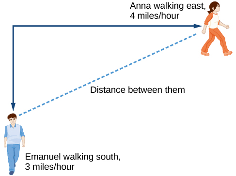
Anna and Emanuel showtime at the same intersection. Anna walks east at four miles per hour while Emanuel walks southward at iii miles per hour. They are communicating with a two-way radio that has a range of two miles. How long later they start walking will they fall out of radio contact?
Solution
In essence, we tin can partially answer this question by saying they will fall out of radio contact when they are 2 miles apart, which leads us to ask a new question:
"How long volition it take them to be 2 miles autonomously?"
In this problem, our irresolute quantities are time and position, but ultimately we need to know how long volition it take for them to be two miles apart. We tin meet that time will be our input variable, so nosotros'll ascertain our input and output variables.
- Input: \(t\), fourth dimension in hours.
- Output: \(A(t)\), distance in miles, and \(Due east(t)\), distance in miles
Because information technology is not obvious how to define our output variable, nosotros'll start by drawing a picture such as Figure \(\PageIndex{three}\).
- Initial Value: They both commencement at the same intersection and so when \(t=0\), the distance traveled by each person should as well be 0. Thus the initial value for each is 0.
- Rate of Change: Anna is walking 4 miles per hour and Emanuel is walking 3 miles per hour, which are both rates of change. The slope for \(A\) is four and the slope for \(Due east\) is iii.
Using those values, we tin can write formulas for the distance each person has walked.
\[A(t)=4t\]
\[E(t)=3t\]
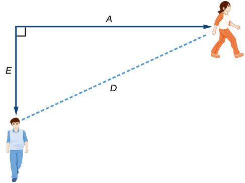
For this problem, the distances from the starting point are important. To notate these, we can define a coordinate organization, identifying the "starting point" at the intersection where they both started. Then nosotros can use the variable, \(A\), which we introduced above, to stand for Anna's position, and define information technology to be a measurement from the starting point in the due east direction. Likewise, tin can use the variable, \(E\), to represent Emanuel's position, measured from the starting point in the due south management. Annotation that in defining the coordinate organisation, we specified both the starting point of the measurement and the direction of measure.
We tin can then define a third variable, \(D\), to exist the measurement of the altitude betwixt Anna and Emanuel. Showing the variables on the diagram is often helpful, as we can see from Figure \(\PageIndex{4}\).
Recall that we need to know how long information technology takes for \(D\), the altitude betwixt them, to equal 2 miles. Notice that for any given input \(t\), the outputs \(A(t)\), \(E(t)\), and \(D(t)\) represent distances.
Using the Pythagorean Theorem, nosotros get:
\[\begin{align*} d(t)^ii&=A(t)^2+E(t)^2 \\ &=(4t)^2+(3t)^2 \\ &=16t^two+9t^2 \\ &=25t^ii \\ D(t)&=\pm\sqrt{25t^2} &\text{Solve for $D(t)$ using the square root} \\ &= \pm 5|t| \end{align*}\]
In this scenario we are because only positive values of \(t\), and then our distance \(D(t)\) volition e'er be positive. We can simplify this respond to \(D(t)=5t\). This ways that the distance between Anna and Emanuel is also a linear role. Because D is a linear role, we can now answer the question of when the distance betwixt them volition reach 2 miles. Nosotros will set the output \(D(t)=2\) and solve for \(t\).
\[\begin{align*} D(t)&=2 \\ 5t&=2 \\ t&=\dfrac{2}{five}=0.four \end{marshal*}\]
They will fall out of radio contact in 0.4 hours, or 24 minutes.
![]() Should I depict diagrams when given information based on a geometric shape?
Should I depict diagrams when given information based on a geometric shape?
Aye. Sketch the figure and label the quantities and unknowns on the sketch.
Example \(\PageIndex{3}\): Using a Diagram to Model Distance betwixt Cities
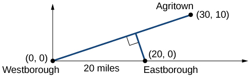
There is a straight route leading from the town of Westborough to Agritown 30 miles east and 10 miles north. Partway downward this road, it junctions with a 2d route, perpendicular to the first, leading to the town of Eastborough. If the town of Eastborough is located 20 miles directly east of the town of Westborough, how far is the route junction from Westborough?
Solution
It might help here to describe a picture of the state of affairs. Encounter Figure \(\PageIndex{5}\). It would then exist helpful to introduce a coordinate system. While we could place the origin anywhere, placing it at Westborough seems user-friendly. This puts Agritown at coordinates \((30, 10)\), and Eastborough at \((20,0)\).
Using this bespeak along with the origin, nosotros tin find the slope of the line from Westborough to Agritown:
\[yard=\dfrac{10-0}{30-0}=\dfrac{1}{3}\]
The equation of the road from Westborough to Agritown would exist
\[Due west(x)=\dfrac{ane}{3}x\]
From this, we can determine the perpendicular road to Eastborough volition have gradient \(thou=–iii\). Because the town of Eastborough is at the indicate \((twenty, 0)\), we can notice the equation:
\[\begin{align*} E(x)&=−3x+b \\ 0&=−three(20)+b &\text{Substitute in $(20, 0)$} \\ b&=lx \\ E(10)&=−3x+60 \finish{marshal*}\]
We tin can now notice the coordinates of the junction of the roads by finding the intersection of these lines. Setting them equal,
\[\begin{align*} \dfrac{ane}{iii}x&=−3x+lx \\ \dfrac{x}{3}ten&=threescore \\ 10x&=180 \\ x&=18 &\text{Substituting this back into $Westward(10)$} \\ y&=W(18) \\ &= \dfrac{i}{3}(18) \\&=6 \end{align*}\]
The roads intersect at the signal \((eighteen,half-dozen)\). Using the distance formula, we can at present find the distance from Westborough to the junction.
\[\begin{align*} \text{distance}&=\sqrt{(x_2-x_1)^2+(y_2-y_1)^ii} \\ &=\sqrt{(eighteen-0)^ii+(6-0)^two} \\ &\approx 18.743 \text{miles} \cease{align*}\]
Assay
I nice utilise of linear models is to take reward of the fact that the graphs of these functions are lines. This means real-world applications discussing maps demand linear functions to model the distances between reference points.
Exercise \(\PageIndex{two}\)
There is a direct road leading from the town of Timpson to Ashburn 60 miles e and 12 miles north. Partway downwardly the road, information technology junctions with a 2d road, perpendicular to the offset, leading to the town of Garrison. If the boondocks of Garrison is located 22 miles directly east of the town of Timpson, how far is the route junction from Timpson?
Solution
21.15 miles
Building Systems of Linear Models
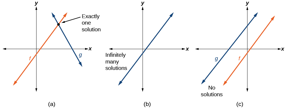
Real-world situations including two or more linear functions may be modeled with a system of linear equations. Retrieve, when solving a arrangement of linear equations, nosotros are looking for points the two lines have in common. Typically, there are three types of answers possible, equally shown in Figure \(\PageIndex{vi}\).
![]() Given a situation that represents a system of linear equations, write the system of equations and identify the solution.
Given a situation that represents a system of linear equations, write the system of equations and identify the solution.
- Place the input and output of each linear model.
- Identify the slope and y-intercept of each linear model.
- Notice the solution by setting the two linear functions equal to another and solving for \(x\),or find the point of intersection on a graph.
Example \(\PageIndex{4}\): Building a System of Linear Models to Choose a Truck Rental Company
Jamal is choosing between 2 truck-rental companies. The first, Keep on Trucking, Inc., charges an up-forepart fee of $20, then 59 cents a mile[1]. The 2d, Move Information technology Your Way, charges an up-front fee of $sixteen, then 63 cents a mile. When volition Keep on Trucking, Inc. be the meliorate choice for Jamal?
Solution
The two important quantities in this problem are the cost and the number of miles driven. Because we have ii companies to consider, we will define 2 functions.
- Input: \(d\), distance driven in miles
- Outputs: \(Grand(d):\) price, in dollars, for renting from Continue on Trucking
\(M(d):\) price, in dollars, for renting from Move It Your Way
- Initial Value: Up-front fee: \(K(0)=xx\) and \(Yard(0)=16\)
- Rate of Change: \(Chiliad(d)=\dfrac{$0.59}{\text{mile}}\) and \(P(d)=\dfrac{$0.63}{\text{mile}}\)
A linear part is of the form \(f(x)=mx+b\). Using the rates of change and initial charges, we can write the equations
\[K(d)=0.59d+20 \nonumber\]
\[M(d)=0.63d+16 \nonumber\]
Using these equations, we tin make up one's mind when Proceed on Trucking, Inc. will be the better choice. Because all we have to make that conclusion from is the costs, we are looking for when Keep on Trucking, Inc. will cost less, or when \(K(d)<M(d)\). The solution pathway volition lead the states to find the equations for the two functions, discover the intersection, and so see where the \(K(d)\) part is smaller.
These graphs are sketched in Figure \(\PageIndex{7}\), with \(Yard(d)\) in blue.
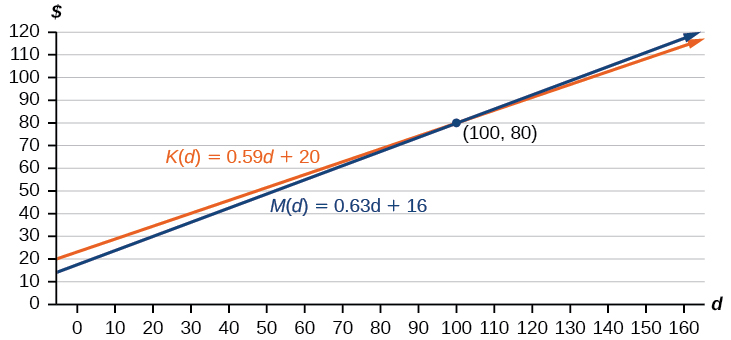
To observe the intersection, nosotros set the equations equal and solve:
\[\begin{align*} K(d)&=M(d) \\ 0.59d+20&=0.63d+16 \\ 4&=0.04d \\ 100&=d \\ d&=100 \end{align*}\]
This tells the states that the cost from the two companies volition be the aforementioned if 100 miles are driven. Either by looking at the graph, or noting that \(One thousand(d)\) is growing at a slower rate, nosotros tin can conclude that Keep on Trucking, Inc. volition be the cheaper price when more than 100 miles are driven, that is \(d>100\).
Central Concepts
- We can use the same problem strategies that we would use for whatever type of function.
- When modeling and solving a trouble, place the variables and look for cardinal values, including the slope and y-intercept.
- Draw a diagram, where appropriate.
- Cheque for reasonableness of the answer.
- Linear models may exist congenital by identifying or calculating the slope and using the y-intercept.
- The ten-intercept may exist found by setting \(y=0\), which is setting the expression \(mx+b\) equal to 0.
- The bespeak of intersection of a organization of linear equations is the signal where the 10- and y-values are the aforementioned.
- A graph of the system may exist used to identify the points where one line falls below (or above) the other line.
Source: https://math.libretexts.org/Bookshelves/Algebra/Map:_College_Algebra_%28OpenStax%29/04:_Linear_Functions/4.03:_Modeling_with_Linear_Functions
0 Response to "Everything You Need to Know About Linear Functions and Modeling Linear Functions"
Post a Comment