Correlation Measures Between Categorical and Continuous Variables
27 mins read
This scenario can happen when we are doing regression or classification in machine learning.
- Regression: The target variable is numeric and one of the predictors is categorical
- Classification: The target variable is categorical and one of the predictors in numeric
In both these cases, the strength of the correlation between the variables can be measured using the ANOVA test. ANOVA stands for Analysis Of Variance. Actually, this test measures if there are any significant differences between the means of the values of the numeric variable for each categorical value. This is something that you can visualize using a box plot as well.
Null hypothesis(H0) ANOVA hypothesis test: The variables are not correlated with each other
In the below example, we are trying to measure if there is any correlation between FuelType on CarPrices. Here FuelType is a categorical predictor and CarPrices is the numeric target variable.
# Generating sample data import pandas as pd ColumnNames=['FuelType','CarPrice'] DataValues= [[ 'Petrol', 2000], [ 'Petrol', 2100], [ 'Petrol', 1900], [ 'Petrol', 2150], [ 'Petrol', 2100], [ 'Petrol', 2200], [ 'Petrol', 1950], [ 'Diesel', 2500], [ 'Diesel', 2700], [ 'Diesel', 2900], [ 'Diesel', 2850], [ 'Diesel', 2600], [ 'Diesel', 2500], [ 'Diesel', 2700], [ 'CNG', 1500], [ 'CNG', 1400], [ 'CNG', 1600], [ 'CNG', 1650], [ 'CNG', 1600], [ 'CNG', 1500], [ 'CNG', 1500] ] #Create the Data Frame CarData=pd.DataFrame(data=DataValues,columns=ColumnNames) print(CarData.head()) ######################################################## # f_oneway() function takes the group data as input and # returns F-statistic and P-value from scipy.stats import f_oneway # Running the one-way anova test between CarPrice and FuelTypes # Assumption(H0) is that FuelType and CarPrices are NOT correlated # Finds out the Prices data for each FuelType as a list CategoryGroupLists=CarData.groupby('FuelType')['CarPrice'].apply(list) # Performing the ANOVA test # We accept the Assumption(H0) only when P-Value > 0.05 AnovaResults = f_oneway(*CategoryGroupLists) print('P-Value for Anova is: ', AnovaResults[1]) Sample Output

As the output of the P-value is almost zero, hence, we reject H0. This means the variables are correlated with each other.
Correlation between two categorical features
This is a situation that arises often during classification machine learning. The target variable is categorical and the predictors can be either continuous or categorical, so when both of them are categorical, then the strength of the relationship between them can be measured using aChi-square test.
The Chi-square test finds the probability of a Null hypothesis(H0).
- Assumption(H0): The two columns are NOT related to each other
- Result of Chi-Sq Test: The Probability of H0 being True
- More information on ChiSq can be found here
It can help to understand whether both the categorical variables are correlated with each other or not. In the below scenario, we try to measure the correlation between GENDER and LOAN_APPROVAL.
# Creating a sample data frame import pandas as pd ColumnNames=['CIBIL','AGE','GENDER' ,'SALARY', 'APPROVE_LOAN'] DataValues=[ [480, 28, 'M', 610000, 'Yes'], [480, 42, 'M',140000, 'No'], [480, 29, 'F',420000, 'No'], [490, 30, 'M',420000, 'No'], [500, 27, 'M',420000, 'No'], [510, 34, 'F',190000, 'No'], [550, 24, 'M',330000, 'Yes'], [560, 34, 'M',160000, 'Yes'], [560, 25, 'F',300000, 'Yes'], [570, 34, 'M',450000, 'Yes'], [590, 30, 'F',140000, 'Yes'], [600, 33, 'M',600000, 'Yes'], [600, 22, 'M',400000, 'Yes'], [600, 25, 'F',490000, 'Yes'], [610, 32, 'M',120000, 'Yes'], [630, 29, 'F',360000, 'Yes'], [630, 30, 'M',480000, 'Yes'], [660, 29, 'F',460000, 'Yes'], [700, 32, 'M',470000, 'Yes'], [740, 28, 'M',400000, 'Yes']] #Create the Data Frame LoanData=pd.DataFrame(data=DataValues,columns=ColumnNames) print(LoanData.head()) ######################################################### # Cross tabulation between GENDER and APPROVE_LOAN CrosstabResult=pd.crosstab(index=LoanData['GENDER'],columns=LoanData['APPROVE_LOAN']) print(CrosstabResult) # importing the required function from scipy.stats import chi2_contingency # Performing Chi-sq test ChiSqResult = chi2_contingency(CrosstabResult) # P-Value is the Probability of H0 being True # If P-Value>0.05 then only we Accept the assumption(H0) print('The P-Value of the ChiSq Test is:', ChiSqResult[1]) Sample Output:
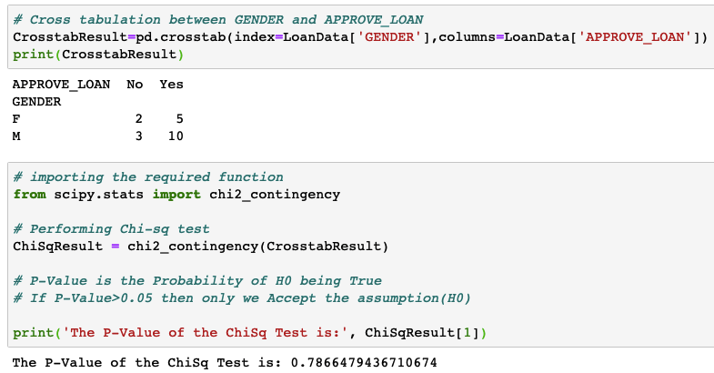
H0: The variables are not correlated with each other. This is the H0 used in the Chi-square test.
In the above example, the p-value came higher than 0.05. Hence H0 will be accepted. This means the variables are not correlated with each other. This means that if two variables are correlated, then the p-value will come very close to zero.
Details of the chi-square test
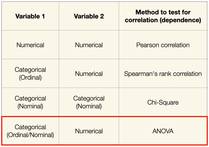
In this section, I will explain how we can test two categorical columns in a dataset to determine if they are dependent on each other (i.e. correlated). We will use a statistics test known aschi-square(commonly written as χ2). Before we start our discussion on chi-square, here is a quick summary of the test methods that can be used for testing the various types of variables:

Using the chi-square statistics to determine if two categorical variables are correlated
Thechi-square (χ2) statistics is a way to check the relationship between two categorical nominal variables . Nominal variables contain values that have no intrinsic ordering. Examples of nominal variables are sex, race, eye color, skin color, etc. Ordinal variables, on the other hand, contain values that are ordered. Examples of ordinal variables are grade, education level, economic status, etc.
The key idea behind the chi-square test is to compare the observed values in the data to the expected values and see if they are related or not. In particular, it is a useful way to check if two categorical nominal variables are correlated. This is particularly important in machine learning where we only want features that are correlated to the target to be used for training.
There are two types of chi-square tests:
- Chi-Square Goodness of Fit Test — test if one variable is likely to come from a given distribution.
- Chi-Square Test of Independence — test if two variables might be correlated or not.
Check out https://www.jmp.com/en_us/statistics-knowledge-portal/chi-square-test.html for a more detailed discussion of the above two chi-square tests. When comparing to see if two categorical variables are correlated, we will use theChi-Square Test of Independence.
Steps to Perform Chi-Square Test
To use the chi-square test, we need to perform the following steps:
- Define thenull hypothesis andalternate hypothesis. They are:
- H₀ (Null Hypothesis) — that the 2 categorical variables being compared areindependent of each other.
- H₁ (Alternate Hypothesis) — that the 2 categorical variables being compared aredependent on each other.
2. Decide on theα value. This is the risk that we are willing to take in drawing the wrong conclusion. As an example, say we setα=0.05 when testing for independence. This means we are undertaking a 5% risk of concluding that two variables are independent when in reality they are not.
3. Calculate thechi-squarescore using the two categorical variables and use it to calculate thep-value. A low p-value means there is a high correlation between two categorical variables (they are dependent on each other). The p-value is calculated from the chi-square score. The p-value will tell if the test results are significant or not.
In a chi-square analysis, the p-value is the probability of obtaining a chi-square as large or larger than that in the current experiment and yet the data will still support the hypothesis. It is the probability of deviations from what was expected being due to mere chance. In general a p-value of 0.05 or greater is considered critical, anything less means the deviations are significant and the hypothesis being tested must be rejected.
Source: https://passel2.unl.edu/view/lesson/9beaa382bf7e/8
To calculate the p-value, we need two pieces of information:
- Degrees of freedom —the number of categories minus 1
- Chi-square score.
If the p-valueobtained is:
- < 0.05 (theα value we have chosen) we reject theH₀ (Null Hypothesis) and accept theH₁ (Alternate Hypothesis). This means the two categorical variables aredependent.
- > 0.05 we accept theH₀ (Null Hypothesis) and reject theH₁ (Alternate Hypothesis). This means the two categorical variables areindependent.
In the case of feature selection for machine learning, we would want the feature that is being compared to the target to have alow p-value (less than 0.05), as this means that the feature is dependent on (correlated to) the target.
With the chi-square score that is calculated, we can also use it to refer to achi-square table to see if the score falls within the rejection region or the acceptance region. In the next we, I will use the Titanic dataset and apply the chi-square test on a few of the features and see how if they are correlated to the target.
Using the chi-square test on the Titanic dataset
A good way to understand a new topic is to go through the concepts using an example. For this, I am going to use the classic Titanic dataset (https://www.kaggle.com/tedllh/titanic-train).
The Titanic dataset is often used in machine learning to demonstrate how to build a machine-learning model and use it to make predictions. In particular, the dataset contains several features (Pclass,Sex,Age,Embarked, etc) and one target (Survived). Several features in the dataset are categorical variables:
- Pclass-the class of cabin that the passenger was in
- Sex-the sex of the passenger
- Embarked-the port of embarkation
- Survived-if the passenger survived the disaster
Because this section explores the relationships between categorical features and targets, we are only interested in those columns that contain categorical values.
Loading the Dataset
Let's load the dataset in a Pandas DataFrame:
import pandas as pd import numpy as np df = pd.read_csv('titanic_train.csv') df.sample(5) 
Data Cleansing and Feature Engineering
There are some columns that are not really useful and hence we will proceed to drop them. Also, there are some missing values so let's drop all those rows with empty values:
df.drop(columns=['PassengerId','Name', 'Ticket','Fare','Cabin'], inplace=True) df.dropna(inplace=True) df 
We will also add one more column namedAlone, based on theParch (Parent or children) andSibsp (Siblings or spouse) columns. The idea we want to explore is if being alone affects the survivability of the passenger. SoAlone is 1 if bothParch andSibsp are 0, else it is 0:
df['Alone'] = (df['Parch'] + df['SibSp']).apply( lambda x: 1 if x == 0 else 0) df 
Visualizing the correlations between features and target
Now that the data is cleaned, let's try to visualize how the sex of passengers is related to their survival in the accident:
import seaborn as sns sns.barplot(x='Sex', y='Survived', data=df, ci=None) The Sex column contains nominal data(i.e. ranking is not important).
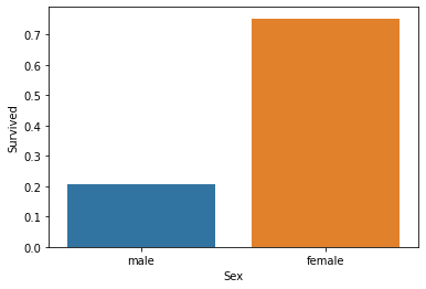
From the above figure, we can see that of all the female passengers, more than 70% survived; of all the men, about 20% survived. Seems like there exists a very strong relationship between Sex andSurvived features. To confirm this, we will use the chi-square test to confirm this later on.
How aboutPclass andSurvived? Are they related?
sns.barplot(x='Pclass', y='Survived', data=df, ci=None) 
Perhaps unsurprisingly, it shows that the higher thePclass that the passenger was in, the higher the survival rate of the passenger. The next feature of interest is if the place of embarkation determines who survives and who doesn't:
sns.barplot(x='Embarked', y='Survived', data=df, ci=None) 
From the chart, it seems like more people who embarked fromC (Cherbourg) survived.
C = Cherbourg; Q = Queenstown; S = Southampton
We also want to know if being alone on the trip makes one more survivable:
ax = sns.barplot(x='Alone', y='Survived', data=df, ci=None) ax.set_xticklabels(['Not Alone','Alone']) 
We can see that if one is with their family, he/she will have a higher chance of survival.
Visualizing the correlations between each feature
Now that we have visualized the relationships between the categorical features against the target (Survived), we want to now visualize the relationships between each feature. Before we can do that, we need to convert the label values in theSex andEmbarked columns to numeric. To do that, we can make use of theLabelEncoder class insklearn:
import numpy as np import pandas as pd import matplotlib.pyplot as plt import seaborn as snsfrom sklearn import preprocessing le = preprocessing.LabelEncoder() le.fit(df['Sex']) df['Sex'] = le.transform(df['Sex']) sex_labels = dict(zip(le.classes_, le.transform(le.classes_))) print(sex_labels) le.fit(df['Embarked']) df['Embarked'] = le.transform(df['Embarked']) embarked_labels = dict(zip(le.classes_, le.transform(le.classes_))) print(embarked_labels) The above code snippet label-encodes theSex andEmbarked columns. The output shows the mappings of the values for each column, which is very useful later when performing predictions:
{'female': 0, 'male': 1} {'C': 0, 'Q': 1, 'S': 2} The following statements show the relationship betweenEmbarked andSex:
ax = sns.barplot(x='Embarked', y='Sex', data=df, ci=None) ax.set_xticklabels(embarked_labels.keys()) 
Seems like more males boarded from Southampton (S) than in Queenstown (Q) and Cherbourg (C).
How aboutEmbarked andAlone?
ax = sns.barplot(x='Embarked', y='Alone', data=df, ci=None) ax.set_xticklabels(embarked_labels.keys()) 
Seems like a large proportion of those who embarked from Queenstown are alone.
And finally, let's see the relationship betweenSex andAlone:
ax = sns.barplot(x='Sex', y='Alone', data=df, ci=None) ax.set_xticklabels(sex_labels.keys()) 
As we can see, there are more males than females who are alone on the trip.
Defining the Hypotheses
We now define thenull hypothesis andalternate hypothesis. As explained earlier, they are:
- H₀ (Null Hypothesis) — that the 2 categorical variables to be compared areindependent of each other.
- H₁ (Alternate Hypothesis) — that the 2 categorical variables being compared aredependent on each other.
And we draw conclusions based on the following p-value conditions:
- p < 0.05 — this means the two categorical variables are correlated .
- p > 0.05 — this means the two categorical variables are not correlated .
Calculating χ2 manually
Let's manually go through the steps in calculating the χ2 values. The first step is to create acontingency table. Using theSex andSurvived columns as an example, we first create a contingency table:

The contingency table above displays the frequency distribution of the two categorical columns —Sex andSurvived.
TheDegrees of Freedom is next calculated as (number of rows -1) * (number of columns -1) . In this example, the degree of freedom is (2–1)*(2–1) =1.
Once the contingency table is created, sum up all the rows and columns, like this:

The above is theObserved values.
Next, we are going to calculate theExpected values. Here is how they are calculated:
- Replace each value in the observed value with the product of the sum of its column and the sum of its row, divided by the total sum.
The following figure shows how the first value is calculated:

The next figure shows how the second value is calculated:

Here is the result for theExpected values:

Then, calculate thechi-square value for each cell using the formula for χ2:

Applying this formula to theObserved andExpected values, we get the chi-square values:

Thechi-square score is the grand total of the chi-square values:

We can use the following websites to verify if the numbers are correct:
- Chi-Square Calculator — https://www.mathsisfun.com/data/chi-square-calculator.html
The Python implementation for the above steps is contained within the followingchi2_by_hand()function:
def chi2_by_hand(df, col1, col2): #---create the contingency table--- df_cont = pd.crosstab(index = df[col1], columns = df[col2]) display(df_cont) #---calculate degree of freedom--- degree_f = (df_cont.shape[0]-1) * (df_cont.shape[1]-1) #---sum up the totals for row and columns--- df_cont.loc[:,'Total']= df_cont.sum(axis=1) df_cont.loc['Total']= df_cont.sum() print('---Observed (O)---') display(df_cont) #---create the expected value dataframe--- df_exp = df_cont.copy() df_exp.iloc[:,:] = np.multiply.outer( df_cont.sum(1).values,df_cont.sum().values) / df_cont.sum().sum() print('---Expected (E)---') display(df_exp) # calculate chi-square values df_chi2 = ((df_cont - df_exp)**2) / df_exp df_chi2.loc[:,'Total']= df_chi2.sum(axis=1) df_chi2.loc['Total']= df_chi2.sum() print('---Chi-Square---') display(df_chi2) #---get chi-square score--- chi_square_score = df_chi2.iloc[:-1,:-1].sum().sum() return chi_square_score, degree_f Thechi2_by_hand() function takes in three arguments — the dataframe containing all columns, followed by two strings containing the names of the two columns we are comparing against. It returns a tuple — the chi-square score, plus the degrees of freedom.
Let's now test the above function using the Titanic dataset. First, let's compare theSex and theSurvived columns:
chi_score, degree_f = chi2_by_hand(df,'Sex','Survived') print(f'Chi2_score: {chi_score}, Degrees of freedom: {degree_f}') Chi2_score: 205.1364846934008, Degrees of freedom: 1 Using the chi-square score, we can now decide if we will accept or reject the null hypothesis using thechi-square distribution curve:

The x-axis represents theχ2 score. The area that is to the right of thecritical chi-square region is known as therejection region. The area to the left of it is known as theacceptance region. If the chi-square score that we have obtained falls in the acceptance region, the null hypothesis is accepted; else the alternate hypothesis is accepted.
So how do we obtain thecritical chi-square region? For this, we have to check thechi-square table:

We can check out theChi-Square Table athttps://www.mathsisfun.com/data/chi-square-table.html
This is how we use the chi-square table. With theα set to be 0.05, and1 degree of freedom, the critical chi-square region is3.84 (refer to the chart above). Putting this value into the chi-square distribution curve, we can conclude that:

- As the calculated chi-square value (205) is greater than3.84, it, therefore, falls in therejection region, and hence the null hypothesis is rejected and thealternate hypothesis is accepted.
- Recalling our alternate hypothesis asH₁ (Alternate Hypothesis) — that the 2 categorical variables being compared aredependent on each other.
This means that the Sex and Survived columns are dependent on each other. We can use the chi2_by_hand() function on the other features.
Calculating the p-value
The previous section shows how we can accept or reject the null hypothesis by examining the chi-square score and comparing it with the chi-square distribution curve. An alternative way to accept or reject the null hypothesis is by using thep-value. Remember, the p-value can be calculated using the chi-square score and the degrees of freedom. For simplicity, we shall not go into the details of how to calculate the p-value by hand.
In Python, we can calculate the p-value using thestats module'ssf() function:
def chi2_by_hand(df, col1, col2): #---create the contingency table--- df_cont = pd.crosstab(index = df[col1], columns = df[col2]) display(df_cont) ... chi_square_score = df_chi2.iloc[:-1,:-1].sum().sum() #---calculate the p-value--- from scipy import stats p = stats.distributions.chi2.sf(chi_square_score, degree_f) return chi_square_score, degree_f, p We can now call thechi2_by_hand() function and get both the chi_square score, degrees of freedom, and p-value:
chi_score, degree_f, p = chi2_by_hand(df,'Sex','Survived') print(f'Chi2_score: {chi_score}, Degrees of freedom: {degree_f}, p-value: {p}') The above code results in the following p-value:
Chi2_score: 205.1364846934008, Degrees of freedom: 1, p-value: 1.581266384342472e-46 As a quick recap, we accept or reject the hypotheses and form the conclusion based on the following p-value conditions:
- p < 0.05 — this means the two categorical variables are correlated .
- p > 0.05 — this means the two categorical variables are not correlated .
And sincep < 0.05 — this means the two categorical variables are correlated .
Trying out the other features
Let's try out the categorical columns that contain nominal values:
chi_score, degree_f, p = chi2_by_hand(df,'Embarked','Survived') print(f'Chi2_score: {chi_score}, Degrees of freedom: {degree_f}, p-value: {p}') # Chi2_score: 27.918691003688615, Degrees of freedom: 2, # p-value: 8.660306799267924e-07 chi_score, degree_f, p = chi2_by_hand(df,'Alone','Survived') print(f'Chi2_score: {chi_score}, Degrees of freedom: {degree_f}, p-value: {p}') # Chi2_score: 28.406341862069905, Degrees of freedom: 1, # p-value: 9.834262807301776e-08 Since the p-values for bothEmbarked andAlone are < 0.05, we can conclude that both theEmbarked andAlone features are correlated to theSurvived target, and should be included for training in our model.
Summary Chi-square
A few notes of caution would be useful here:
- While thePearson's coefficient andSpearman's rank coefficient measure thestrength of an association between two variables, thechi-square test measures thesignificance of the association between two variables. What it tells us is whether the relationship we found in the sample is likely to exist in the population, or how likely it is by chance due to sampling error.
- Thechi-square test is sensitive to small frequencies in the contingency table. Generally, if a cell in the contingency table has a frequency of 5 or less, the chi-square test will lead to errors in the conclusion. Also, the chi-square test should not be used if the sample size is less than 50.
Details of ANOVA
The chi-square test is used when both the independent and dependent variables are allcategorical variables. However, what if the independent variable iscategorical and the dependent variable isnumerical? In this case, we have to use another statistic test known as ANOVA —AnalysisofVariance.
And so in this section, our discussion will revolve around ANOVA and how we use it in machine learning for feature selection. Before we get started, it is useful to summarize the different methods that we have discussed so far:
What is ANOVA?
ANOVA is used for testing two variables, where:
- one is acategorical variable
- another is anumerical variable
ANOVA is used when the categorical variable hasat least 3 groups (i.e three different unique values). If we want to compare just two groups, we use the t-test. ANOVA lets us know if a numerical variable changes according to the level of the categorical variable. ANOVA uses the f-tests to statistically test the equality of means. F-tests are named after their test statistic, F, which was named in honor ofSir Ronald Fisher.
Here are some examples that make it easier to understand when we can use ANOVA.
We have a dataset containing information about a group of people pertaining to their social media usage and the number of hours they sleep:

We want to find out if the amount of social media usage (categorical variable) has a direct impact on the number of hours of sleep (numerical variable).
We have a dataset containing three different brands of medication and the number of days for the medication to take effect:

We want to find out if there is a direct relationship between a specific brand and its effectiveness.
ANOVA checks whether there is equal variance between groups of categorical features with respect to the numerical response. If there is equal variance between groups, it means this feature has no impact on the response and hence it (the categorical variable) cannot be considered for model training.
Performing AVONA by hand
The best way to understand ANOVA is to use an example. In the following example, I use a fictitious dataset where I recorded the reaction time of a group of people when they are given a specific type of drink.
Sample Dataset
I have a sample dataset nameddrinks.csv containing the following content:
team,drink_type,reaction_time 1,water,14 2,water,25 3,water,23 4,water,27 5,water,28 6,water,21 7,water,26 8,water,30 9,water,31 10,water,34 1,coke,25 2,coke,26 3,coke,27 4,coke,29 5,coke,25 6,coke,23 7,coke,22 8,coke,27 9,coke,29 10,coke,21 1,coffee,8 2,coffee,20 3,coffee,26 4,coffee,36 5,coffee,39 6,coffee,23 7,coffee,25 8,coffee,28 9,coffee,27 10,coffee,25 There are 10 teams in all — each team comprises 3 persons. Each person in the team is given three different types of drinks — water, coke, and coffee. After consuming the drink, they were asked to perform some activities and their reaction time was recorded. The aim of this experiment is to determine if the drinks have any effect on a person's reaction time.
Let's first load the dataset into a Pandas DataFrame:
import pandas as pd df = pd.read_csv('drinks.csv') Record theobservation size, which we will make use of later:
observation_size = df.shape[0] # number of observations 
Visualizing the dataset
It is useful to visualize the distribution of the data using a Boxplot:
_ = df.boxplot('reaction_time', by='drink_type') 
We can see that the three types of drinks have about the same median reaction time.
Pivoting the dataframe
To facilitate the calculation for ANOVA, we need to pivot the dataframe:
df = df.pivot(columns='drink_type', index='team') display(df) 
The columns represent the three different types of drinks and the rows represent the 10 teams. We will also use this chance to record thenumber of items in each group, as well as thenumber of groups, which we will make use of later:
n = df.shape[0] # 10; number of items in each group k = df.shape[1] # 3; number of groups 
Defining the Hypotheses
We now define thenull hypothesis andalternate hypothesis, just like the chi-square test. They are:
- H₀ (Null hypothesis) — that there is no difference among group means.
- H₁ (Alternate hypothesis) — that at least one group differs significantly from the overall mean of the dependent variable.
Step 1 — Calculating the means for all groups
We are now ready to begin our calculations for ANOVA. First, let's find the mean for each group:
df.loc['Group Means'] = df.mean() df 
From here, we can now calculate theoverall mean:
overall_mean = df.iloc[-1].mean() overall_mean # 25.666666666666668 
Step 2 — Calculate the Sum of Squares
Now that we have calculated theoverall mean, we can proceed to calculate the following:
- Sum of squares of all observations —SS_total
- Sum of squares within —SS_within
- Sum of squares between —SS_between
Sum of squares of all observations —SS_total
Thesum of squares of all observations is calculated by deducting each observation from theoverall mean, and then summing all the squares of the differences:


Programmatically,SS_total is computed as:
SS_total = (((df.iloc[:-1] - overall_mean)**2).sum()).sum() SS_total # 1002.6666666666667 Sum of squares within — SS_within
Thesum of squares within is the sum of squared deviations of scores around their group's mean:

Programmatically,SS_within is computed as:
SS_within = (((df.iloc[:-1] - df.iloc[-1])**2).sum()).sum() SS_within # 1001.4 Sum of Squares between — SS_between
Next, we calculate the sum of squares of the group means from the overall mean:


Programmatically,SS_between is computed as:
SS_between = (n * (df.iloc[-1] - overall_mean)**2).sum() SS_between # 1.266666666666667 We can verify that:
SS_total =SS_between +SS_within
Creating the ANOVA Table
With all the values computed, we can now complete the ANOVA table. Recall we have the following variables:

We can compute the variousdegrees of freedoms as follows:
df_total = observation_size - 1 # 29 df_within = observation_size - k # 27 df_between = k - 1 # 2 From the above, compute the variousmean squared values:
mean_sq_between = SS_between / (k - 1) # 0.6333333333333335 mean_sq_within = \ SS_within / (observation_size - k) # 37.08888888888889 Finally, we can calculate theF-value, which is the ratio of two variances:
F = mean_sq_between / mean_sq_within # 0.017076093469143204 Recall earlier that I mentioned ANOVA uses the f-tests to statistically test the equality of means.
Once the F-value is obtained, we now have to refer to thef-distribution table(see http://www.socr.ucla.edu/Applets.dir/F_Table.html for one example) to obtain thef-critical value. The f-distribution table is organized based on theα value (usually 0.05). So we need to first locate the table based onα=0.05:

Next, observe that the columns of the f-distribution table are based ondf1 while the rows are based ondf2. We can getdf1 anddf2 from the previous variables that we have created:
df1 = df_between # 2 df2 = df_within # 27 Using the values ofdf1 anddf2, we can now locate thef-critical value by locating thedf1 column anddf2 row:

From the above figure, we can see that thef-critical value is3.3541. Using this value, we can now decide if we will accept or reject the null hypothesis using theF-distribution curve:

Since thef-value (0.0171, which is what we can calculate) is less than the f-critical value in the f-distribution table, we accept the null hypothesis —this means there is no variance in different groups — all the means are the same. For machine learning, this feature —drink_type, should not be included for training as it seems the different types of drinks have no effect on the reaction time. We should only include a feature for training only if we reject the null hypothesis as this means that the values in the drink types affect on the reaction time.
Using the Stats module to calculate f-score
In the previous section, we manually calculated the f-value for our dataset. Actually, there is an easier way — use thestats module'sf_oneway() function to calculate the f-value and p-value:
import scipy.stats as stats fvalue, pvalue = stats.f_oneway( df.iloc[:-1,0], df.iloc[:-1,1], df.iloc[:-1,2]) print(fvalue, pvalue) # 0.0170760934691432 0.9830794846682348 Thef_oneway() function takes the groups as input and returns the ANOVA F and p-value:

In the above, thef-value is0.0170760934691432 (identical to the one we calculated manually) and thep-value is0.9830794846682348.
Observe that thef_oneway() function takes in a variable number of arguments:

If we have many groups, it would be quite tedious to pass in the values of all the groups one by one. So, there is an easier way:
fvalue, pvalue = stats.f_oneway( *df.iloc[:-1,0:3].T.values ) Using the statsmodels module to calculate f-score
Another way to calculate the f-value is to use thestatsmodel module. We first build the model using theols() function, and then call thefit() function on the instance of the model. Finally, we call theanova_lm() function on the fitted model and specify the type of ANOVA test to perform on it. There are 3 types of ANOVA tests to perform, but their discussion is beyond the scope of this article.
import pandas as pd import statsmodels.api as sm from statsmodels.formula.api import ols df = pd.read_csv('drinks.csv') model = ols('reaction_time ~ drink_type', data=df).fit() sm.stats.anova_lm(model, typ=2) The above code snippet produces the following result, which is the same as the f-value that we calculated earlier (0.017076):

Theanova_lm() function also returns the p-value (0.983079). We can make use of the following rules to determine if the categorical variable has any influence on the numerical variable:
- if p < 0.05, this means that the categorical variable has a significant influence on the numerical variable
- if p > 0.05, this means that the categorical variable has no significant influence on the numerical variable
Since the p-value is now 0.983079 (>0.05), this means that thedrink_type has no significant influence on thereaction_time.
Summary of ANOVA
ANOVA helps to determine if a categorical variable has an influence on a numerical variable. So far the ANOVA test that we have discussed is known as theone-way ANOVA test. There are a few variations of ANOVA:
- One-way ANOVA— is used to check how a numerical variable responds to the levels of one independent categorical variables
- Two-way ANOVA —is used to check how a numerical variable responds to the levels oftwo independent categorical variables
- Multi-way ANOVA — is used to check how a numerical variable responds to the levels ofmultiple independent categorical variables
Using atwo-way ANOVA ormulti-way ANOVA, we can investigate the combined impact of two (or more) independent categorical variables on one dependent numerical variable.
Resources:
https://thinkingneuron.com/how-to-measure-the-correlation-between-a-numeric-and-a-categorical-variable-in-python/
https://towardsdatascience.com/statistics-in-python-using-chi-square-for-feature-selection-d44f467ca745
https://towardsdatascience.com/statistics-in-python-using-anova-for-feature-selection-b4dc876ef4f0
Source: http://sefidian.com/2021/07/02/measure-the-correlation-between-numerical-and-categorical-variables-and-the-correlation-between-two-categorical-variables-in-python-chi-square-and-anova/
0 Response to "Correlation Measures Between Categorical and Continuous Variables"
Post a Comment